Game Theory: Mixed-Strategies and Zero-Sum Games

I. Introduction
In my previous blog entry, the normal form game and Nash equilibrium were introduced. Attention was restricted to pure strategies. As will be illustrated below, not every finite, normal form game has a pure strategies Nash equilibrium. The notion of mixed strategies extends the notion of pure strategies, allowing players to assign probabilities to each pure strategy. This extension provides for the existence of a mixed strategies Nash equilibrium in every finite, normal form game. Additionally, zero sum games and prudent strategies will be discussed.

II. Mixed-Strategies
In this section, we introduce the notion of mixed-strategies. One important motivator for mixed-strategies is that not every game has a pure strategies Nash equilibrium. Consider the matching pennies game:

Matching_Pennies

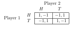
In any pure strategy profile, one player incurs utility $1$ and the other player incurs utility $-1$ . The player incurring utility $-1$ can unilaterally deviate by switching its choice to improve its utility. This inverts the payoffs- the first player incurs utility $-1$ while the second player incurs utility $1$ . Iterating on the above argument, we see that no Nash equilibrium exists in pure strategies.

Mixed Strategies: Let $\Gamma$ be a normal form game. Let $i \in N$ . A mixed strategy is a sequence $(s_{j})_{j=1}^{k} \in S_{i}$ and a probability distribution $\sigma = (\sigma_{j})_{j=1}^{k}$ where player $i$ selects strategy $s_{j}$ with probability $\sigma_{j}$ . Note that $\sum_{j=1}^{k} \sigma_{j} = 1$ . The set of mixed strategies for player $i$ is denoted $\Sigma_{i} := \Delta(S_{i})$ , where $\Delta(S_{i})$ is the simplex in $\mathbb{R}^{|S_{i}|}$ . That is, $\Delta(S_{i}) = \{ x \in \mathbb{R}^{|S_{i}|} : x_{i} \geq 0 \text{ } \forall{i} \in \{1, ..., |S_{i}|\}, \sum_{i=1}^{|S_{i}|} x_{i} = 1 \}$ .

Note that pure strategies are a special case of mixed strategies. The mixed extension will now be defined, to formalize the notion of games with mixed strategies. A mixed strategies Nash equilibrium in a normal form game is equivalent to a pure strategies Nash equilibrium in a mixed extension.

Mixed Extension: Let $\Gamma = [N, (S_{i})_{i \in N}, (u_{i})_{i \in N}]$ be a normal form game. The mixed extension of $\Gamma$ is the three-tuple $[N, (\Sigma_{i})_{i \in N}, (u_{i})_{i \in N}]$ , where $\Sigma_{i} := \Delta(S_{i})$ .

The notion of mixed strategies is rather unintuitive from a behavioral perspective, as a normal form game is played simultaneously. So how is a mixed strategies Nash equilibrium formulated? Recall that each player is a rational, utility maximizing agent that is aware of the structure of the game. Each player still seeks to mix its strategies in such a way to maximize its utility. In mixing strategies, a player runs the risk that another player can take advantage of a given mixing. Thus, in a Nash equilibrium, each player $i$ mixes strategies such that $-i$ is indifferent to whichever pure strategy ends up being played. That is, $-i$ ‘s expected utility for each of $i$ ‘s pure strategies in the mixing is the same. This is formalized as follows.

Theorem 2.1: Let $\Gamma$ be a normal form game. A mixed strategy profile $\sigma^{*}$ is a mixed strategy Nash equilibrium if and only if, for each player $i$ , the following two conditions are satisfied:

Every pure strategy $s_{i} \in S_{i}$ which is given positive probability by $\sigma_{i}^{*}$ yields the same expected payoff against $\sigma_{-i}^{*}$ ; that is, $u_{i}(s_{i}, \sigma_{-i}^{*}) = u_{i}(\sigma^{*})$ .
Every pure strategy $s_{i} \in S_{i}$ which is given probability zero by $\sigma_{i}^{*}$ yields no more than the pure strategies that are assigned positive probability: $u_{i}(s_{i}, \sigma_{-i}^{*}) \leq u_{i}(\sigma^{*})$ .

Proof: Suppose first that the mixed-strategy profile $\sigma^{*}$ satisfies conditions (1) and (2). Let $i \in N$ . If $i$ unilaterally deviates by shifting positive probability to a strategy $s_{i} \in S_{i}$ given zero probability in $\sigma^{*}$ , then $i$ ‘s utility does not increase by condition (2). Let $S_{i}^{\prime} = \{ s_{i} \in S_{i} : \sigma_{i}^{*}(s_{i}) > 0 \}$ be the set of strategies given positive probability by $\sigma_{i}^{*}$ . By condition (1), each pure strategy in $S_{i}^{\prime}$ results in the same expected utility $\overline{u}$ . Thus, any mixing $\gamma$ of strategies in $S_{i}^{\prime}$ results in expected utility:

$\sum_{s_{i} \in S_{i}^{\prime}} \gamma(s_{i}) u_{i}(s_{i}, \sigma_{-i}^{*}) = \overline{u} \sum_{s_{i} \in S_{i}^{\prime}} \gamma(s_{i}) = \overline{u}$

Thus, player $i$ cannot unilaterally deviate and improve its outcome, so $\sigma^{*}$ is a mixed strategies Nash equilibrium.

Conversely, suppose $\sigma^{*}$ is a mixed-strategies Nash equilibrium. As no player can unilaterally deviate and improve its outcome, condition (2) follows immediately. Suppose to the contrary that condition (1) does not hold. Let $i \in N$ and $s_{i} \in S_{i}$ such that the $u_{i}(s_{i}, \sigma_{-i}^{*}) \neq u_{i}(\sigma^{*})$ . If $u_{i}(s_{i}, \sigma_{-i}^{*}) > u_{i}(\sigma^{*})$ , then player $i$ could assign more weight to $s_{i}$ in $\sigma_{i}^{*}$ and improve its outcome. Similarly, if $u_{i}(s_{i}, \sigma_{-i}^{*}) < u_{i}(\sigma^{*})$ , then player $i$ could assign less weight to $s_{i}$ in $\sigma_{i}^{*}$ and improve its outcome. Either occurrence contradicts the assumption that $\sigma^{*}$ is a mixed-strategies Nash equilibrium. QED.

Example 1: Let’s now use Theorem 2.1 to find a mixed-strategies Nash equilibrium for the Matching Pennies game. Player $1$ mixes strategies such that Player $2$ is indifferent to $H$ and $T$ . Suppose Player $1$ plays $H$ with probability $p$ and $T$ with probability $1-p$ . Player $2$ ‘s payoff from playing $H$ is $-p + (1-p) = 1 - 2p$ . Player $2$ ‘s payoff from playing $T$ is $p - (1 - p) = 1-2p$ . In equilibrium, Player $2$ is indifferent between playing $H$ and $T$ . Setting $1 - 2p = 2p - 1 \implies p^{*} = \frac{1}{2}$ . By symmetry, we have Player $2$ mixing between $H$ and $T$ with frequencies $(\frac{1}{2}, \frac{1}{2})$ as well.

In addition to guaranteeing the existence of a Nash equilibrium, mixed strategies are also useful in selecting realistic Nash equilibria. Consider the following example.

Example 2: Consider a traffic routing game on the following network. The weight of each edge denotes the latency cost of traversing that edge. The variable $x$ denotes the number of players traversing the edge $(A, B)$ , and the variable $y$ denotes the number of players using the edge $(C, D)$ . So for example, if $x = 50$ , then the latency cost of $(A, B)$ is $1.5$ for every each of the $50$ players. Each player starts at $A$ and ends at $D$ , seeking to minimize latency.

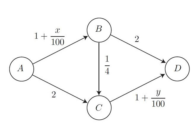
Suppose there are $100$ players in the game. Denote $n_{1}$ as the number of players choosing the path $\text{ABD}$ , $n_{2}$ as the number of players choosing the path $\text{ACD}$ , and $n_{3}$ as the number of players choosing $\text{ABCD}$ . Consider first the pure strategies Nash equilibrium of $n_{1} = 25, n_{2} = 25, n_{3} = 50$ . Both the edges $(A, B)$ and $(C, D)$ have $75$ players traversing them, and so have latency costs $1.75$ . Players of each type incur latency cost $3.75$ . If a player of type $n_{1}$ unilaterally deviates, he increases the latency cost of the edge $(C, D)$ to $1.76$ , resulting in a total latency cost of $3.76$ . By similar argument, players of type $n_{2}$ and $n_{3}$ cannot unilaterally deviate and decrease their costs as well.

While $n_{1} = n_{2} = 25$ and $n_{3} = 50$ is a pure strategies Nash equilibrium, it is unlikely the $100$ players will end up playing this strategy profile. However, this pure strategies equilibrium does provide the probabilities for a mixed strategies equilibrium. As the game is symmetric, there exists a Nash equilibrium in which each player selects the same strategy. Suppose each player selects the mixed strategy $(\text{ABD}, \text{ACD}, \text{ABCD})$ with probabilities $(\frac{1}{4}, \frac{1}{4}, \frac{1}{2})$ . We apply Theorem 2.1 to verify this mixed strategy profile, denoted $\sigma^{*}$ , is a mixed-strategies Nash equilibrium.

First, observe that $\mathbb{E}[u_{i}(\sigma^{*})] = 3.75$ . Consider each of the pure strategies $\text{ABD}, \text{ACD}, \text{ABCD}$ .

Suppose player $i$ plays the pure strategy $\text{ABD}$ . Under $\sigma_{-i}^{*}$ , $n_{1} = 24$ , $n_{2} = 25$ , and $n_{3} = 50$ . So $\mathbb{E}[u_{i}(\text{ABD}, \sigma_{-i}^{*})] = 1.75 + 2 = 3.75 = \mathbb{E}[u_{i}(\sigma^{*})]$ .
Suppose player $i$ plays the pure strategy $\text{ACD}$ . Under $\sigma_{-i}^{*}$ , $n_{1} = 25, n_{2} = 24$ , and $n_{3} = 50$ . So $\mathbb{E}[u_{i}(\text{ACD}, \sigma_{-i}^{*})] = 1.75 + 2 = 3.75 = \mathbb{E}[u_{i}(\sigma^{*})]$ .
Suppose player $i$ plays the pure strategy $\text{ABCD}$ . Under $\sigma_{-i}^{*}$ , $n_{1} = n_{2} = 25$ and $n_{3} = 49$ . So $\mathbb{E}[u_{i}(\text{ABCD}, \sigma_{-i}^{*})] = 1.75 + 0.25 + 1.75 = 3.75 = \mathbb{E}[u_{i}(\sigma^{*})]$ .

Thus, $\sigma^{*}$ is a mixed-strategies Nash equilibrium.

III. Zero-Sum Games
In this section, we examine zero-sum games. Intuitively, in a zero sum game, each player’s gain (or loss) is exactly balanced with those of the other players. For example, cutting a larger slice of cake for one person leaves less cake for the others. This notion is formalized as follows:

Zero-Sum Games: Let $\Gamma$ be a normal form game. $\Gamma$ is said to be a Zero-Sum Game if $\sum_{i \in N} u_{i}(\sigma) = 0$ for every strategy profile $\sigma$ .

Recall the Matching Pennies game from the previous section. In any strategy profile, one player earns utility $1$ while the other player earns utility $-1$ . Thus, the Matching Pennies game is a zero-sum game. Another example of a zero-sum game is Rock-Paper-Scissors. The winner of the game earns utility $1$ while the loser earns utility $-1$ . In the event of a tie, each player earns utility $0$ .

So how are zero-sum games solved? We can solve zero-sum games in the same manner as any other normal form game. Of particular interest, however, areprudent strategies. Intuitively, players who play prudently seek to minimize potential losses. We define prudent strategies as follows:

Prudent Strategies: Let $\Gamma$ be a finite, normal form game. A prudent strategy of player $i$ is a mixed strategy $\sigma_{i}^{*}$ that satisfies $\max_{\sigma_{i}} \min_{\sigma_{-i}} u_{i}(\sigma_{i}, \sigma_{-i})$ .

Note that the definition of prudent strategies did not restrict to zero-sum games. We discuss them in the context of zero-sum games; however, as they are most useful here. In the case of a two-player game, saddle points are equivalent to prudent strategies. We define a saddle point as follows.

Saddle Point: Let $\Gamma$ be a two-player zero-sum game. A saddle point is a strategy profile $(\sigma_{1}^{*}, \sigma_{2}^{*}) \in S_{1} \times S_{2}$ satisfying $u_{i}(\sigma_{1}, \sigma_{2}^{*}) \leq u_{i}(\sigma_{1}^{*}, \sigma_{2}^{*}) \leq u_{i}(\sigma_{1}^{*}, \sigma_{2})$ for all $\sigma_{1} \in S_{1}$ , all $\sigma_{2} \in S_{2}$ , and each $i \in \{1, 2\}$ .

In order to test for saddle points in finite games, we convert the payoff matrix into a mathematical matrix from linear algebra. As we are considering zero sum games, define the matrix $A$ to be a real-valued $|S_{1}| \times |S_{2}|$ matrix where $[A_{ij}] = u_{i}(s_{i}, s_{j})$ , $s_{i} \in S_{1}, s_{j} \in S_{2}$ . That is, $[A_{ij}]$ represents the amount Player 1 wins and Player 2 loses when the pure strategy profile $(s_{i}, s_{j})$ is played. A saddle point $A_{ij}$ is a minimum of row $i$ and a maximum of column $j$ . Let’s consider an example of finding a saddle point.

Example 3: Consider the two-player, zero-sum game given by the following payoff matrix.

Ex3

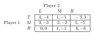
We begin by converting the payoff matrix to an algebraic matrix:

$\begin{bmatrix} 4 & 1 & -3 \\ 3 & 2 & 5 \\ 0 & 1 & 6 \end{bmatrix}$

The row minima are $-3, 2, 0$ ; and the column maxima are $4, 2, 6$ . Observe that row two and column two have the same value: $2$ . So $(M, M)$ is a saddle point with payoff $(2, -2)$ .

Example 4: Consider the two-player, zero-sum game given by the following payoff matrix.

Ex4

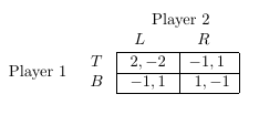
We begin by converting the payoff matrix to an algebraic matrix:

$\begin{bmatrix} 2 & -1 \\ -1 & 1 \end{bmatrix}$

The row minima are $-1$ for row one, and $-1$ for column one. The column maxima are $2$ for column one, and $1$ for column two. So there are no pure strategy saddle points for this game.

We solve this game by determining the mixed strategies Nash equilibria. Suppose Player 2 plays $L$ with probability $p$ and $R$ with probability $(1-p)$ . If Player 1 plays $T$ , his expected payoff is $2p - (1-p) = 3p - 1$ . If Player 1 plays $B$ , his expected payoff is $-p + (1-p) = 1 - 2p$ . Setting $3p - 1 = 1 - 2p \implies p = \frac{2}{5}$ . So Player 2 plays $L$ with probability $\frac{2}{5}$ and $R$ with probability $\frac{3}{5}$ in equilibrium.

We now solve for Player 1’s mixed equilibrium strategies. Suppose Player 1 plays $T$ with probability $q$ and $B$ with probability $1-q$ . Then Player 2’s expected payoff from playing $L$ is $-2q + 1-q = 1 - 3q$ . Player 2’s expected payoff from playing $R$ is $q - (1-q) = 2q - 1$ . Setting $2q - 1 = 1 - 3q$ yields $q = \frac{2}{5}$ . So Player 1 plays $T$ with probability $\frac{2}{5}$ and $B$ with probability $\frac{3}{5}$ in equilibrium.

When considering mixed strategies or infinite games with compact (closed and bounded) strategy sets (such as mixed extensions of normal form games), saddle points are guaranteed to exist. This is due to a result in real analysis known as the Weierstrass Extreme Value Theorem, which states that a continuous function over a compact set achieves both a maximum and a minimum.

It is easy to verify that a pure-strategy saddle point is a Nash equilibrium in a finite zero-sum games. This verification is presented in the following theorem to build intuition. The logic is analogous in the case of infinite games (such as mixed extensions of finite zero-sum games).

Theorem 3.1: Let $\Gamma$ be a two-player zero-sum game and let $A$ be the associated matrix. Suppose $(s_{i}, s_{j}) \in S_{1} \times S_{2}$ is a saddle point. Then $(s_{1}, s_{2})$ constitutes a Nash equilibrium of $\Gamma$ .

Proof: As $A_{ij}$ is the maximum of column $j$ , a unilateral deviation from Player 1 will result in payoff $A_{kj}$ for some $k$ . It follows that $A_{kj} \leq A_{ij}$ , so Player 1 cannot unilaterally deviate and improve its outcome. For Player 2, $u_{2}(s_{i}, s_{j}) = -A_{ij}$ as $\Gamma$ is a zero-sum game and by construction of the matrix $A$ . So if Player 2 unilaterally deviates, the payoff will be $u_{2}(s_{i}, s_{m}) = -A_{im} \leq u_{2}(s_{i}, s_{j})$ since $A_{im} \geq A_{ij}$ . And so Player 2 cannot unilaterally deviate and improve its outcome. Thus, $(s_{i}, s_{j})$ is a Nash equilibrium. QED.

The Nash equilibria of zero-sum games can be characterized in terms of prudent strategies. Intuitively, each player seeks to minimize its opponent’s payoff. As a zero-sum game is being considered, this leaves more for the individual. This notion is formalized as follows:

Theorem 3.2: In any finite, two-person zero-sum game, the following conditions hold:

If $(\sigma_{1}^{*}, \sigma_{2}^{*})$ is a mixed strategies Nash equilibrium, then $\sigma_{i}^{*}$ is a prudent strategy of player $i \in \{1, 2\}$ and: $\max_{\sigma_{1}} \min_{\sigma_{2}} u_{1}(\sigma_{1}, \sigma_{2}) = \min_{\sigma_{2}} \max_{\sigma_{1}} u_{1}(\sigma_{1}, \sigma_{2}) = u_{1}(\sigma_{1}^{*}, \sigma_{2}^{*})$ (2)
If $\sigma_{i}^{*}$ is prudent for each $i \in \{1, 2\}$ , then $(\sigma_{1}^{*}, \sigma_{2}^{*})$ is a mixed-strategies Nash equilibrium.

Proof: Suppose first that $(\sigma_{1}^{*}, \sigma_{2}^{*})$ is a mixed strategies Nash equilibrium. Now suppose to the contrary that for some $i \in \{1, 2\}$ , $\sigma_{i}^{*}$ is not prudent. It follows that there exists a strategy $\sigma_{i}^{\prime}$ guaranteeing a better result than $\sigma_{i}^{*}$ . Consider the mixed strategy profile $(\sigma_{i}^{\prime}, \sigma_{-i}^{\prime})$ , where $\sigma_{-i}^{\prime}$ is a best response to $\sigma_{i}^{\prime}$ . We thus have $u_{i}(\sigma_{i}^{\prime}, \sigma_{-i}^{\prime}) > u_{i}(\sigma_{i}^{*}, \sigma_{-i}^{*})$ . As $\sigma_{i}^{*}$ is a best response to $\sigma_{-i}^{*}$ , we have $u_{i}(\sigma^{*}, \sigma_{-i}^{*}) \geq u_{i}(\sigma_{i}^{\prime}, \sigma_{-i}^{*})$ . As $\sigma_{-i}^{\prime}$ is a best response to $\sigma_{i}^{\prime}$ and the game is zero-sum, it follows that $u_{i}(\sigma_{i}^{\prime}, \sigma_{-i}^{*}) \geq u_{i}(\sigma_{i}^{\prime}, \sigma_{-i}^{\prime})$ . Chaining the inequalities together implies $u_{i}(\sigma_{i}^{\prime}, \sigma_{-i}^{\prime}) > u_{i}(\sigma_{i}^{\prime}, \sigma_{-i}^{\prime})$ , a contradiction. It follows that $\sigma_{i}^{*}$ is prudent for both players.

It will now be shown that (2) holds. Note that for any function $f(x, y)$ and fixed $x, y$ , we have $\min_{y^{\prime}} f(x, y^{\prime}) \leq f(x, y) \leq \max_{x^{\prime}} f(x^{\prime}, y)$ . Taking the max of both sides maintains this inequality. Thus:

$\max_{\sigma_{1}} \min_{\sigma_{2}} u_{1}(\sigma_{1}, \sigma_{2}) \leq \min_{\sigma_{2}} \max_{\sigma_{1}} u_{1}(\sigma_{1}, \sigma_{2})$

Similarly, as $(\sigma_{1}^{*}, \sigma_{2}^{*})$ is a saddle point, we have:

$\max_{\sigma_{1}} u_{1}(\sigma_{1}, \sigma_{2}^{*}) \leq u_{1}(\sigma_{1}^{*}, \sigma_{2}^{*}) \leq \min_{\sigma_{2}} u_{1}(\sigma_{1}^{*}, \sigma_{2})$

And so:

$\min_{\sigma_{2}} \max_{\sigma_{1}} u_{1}(\sigma_{1}, \sigma_{2}) \leq \max_{\sigma_{1}} u_{1}(\sigma_{1}, \sigma_{2}^{*}) \leq \min_{\sigma_{2}} u_{1}(\sigma_{1}^{*}, \sigma_{2}) \leq \max_{\sigma_{1}} \min_{\sigma_{2}} u_{1}(\sigma_{1}, \sigma_{2}^{*})$

Thus, (2) holds.

Conversely, suppose $\sigma_{i}^{*}$ is prudent for each $i \in \{1, 2\}$ . As $\sigma_{i}^{*}$ is prudent, it solves $\max_{\sigma_{i}} u_{i}(\sigma_{i}, \sigma_{-i}^{*})$ . So player $i$ cannot unilaterally deviate and improve its payoff. Thus, $(\sigma_{1}^{*}, \sigma_{2}^{*})$ is a mixed-strategies Nash equilibrium. QED.

Source: Game Theory: Mixed-Strategies and Zero-Sum Games

Forwardeconomics

An evolutionary think tank